# Install and Load Packages

# Downloading all desired packages into local device
install.packages ("tidyverse", repos = "https://cran.rstudio.com") #This package allows for simplified and more intuitive syntax in R
install.packages ("rstatix", repos = "https://cran.rstudio.com") #This package allows for a variety of tests for statistical significance with the use of its integrated functions
install.packages ("ggplot2", repos = "https://cran.rstudio.com") #This package allows for the

# Loading all libraries into current R notebook
library (tidyverse)
library (rstatix)
library (ggplot2)Altitude Associated Changes in ant Morphology and Genus-dependent Resource Preference in Guadarrama Ants
This analysis is based on a several studies taking place in the Guadarra Mountains of Spain by the same group of scientists. Scientists measured the size of the different morphological structures of a multitude of ant genera across varying altitudes and regions of Guadarra mountain range as well as the resources ants were observed using. We aim to analyze how the size of the measured morphological features varies with altitude as well as to understand a genus-specific preference for certain resource types across ant taxa.
The data sets we used can be found here:The original research papers can be found here:
- Diverging facets of grassland ant diversity along a Mediterranean elevational gradient
- Author(s): Mariola Silvestre, Carlos Carmona, Francisco Azcárate, Javier Seoane.
- Abiotic controls, but not species richness, shape niche overlap and breadth of ant assemblages along an elevational gradient in central Spain
- Author(s): Javier Seoane, Mariola Silvestre, Violeta Hevia, Rubén Ariño and Francisco Azcárate.
Figure 1: Image of ___ (Aphaenogaster gibbosa) consuming deceased insect.
Data Analysis
The following scripts are used to answer two hypothesis we
Hypothesis 1:
Data Summary Calculations
# Import Data + Create Dataframes

Ant = read.csv("Ant_traits_in_central_Spain.csv", header = TRUE) #Importing data set into R from local device for Hypothesis 1

head_mean = mean(Ant$head) #Create data frame for the mean size of ant head
print(head_mean) #Output the value in 'head_mean', the mean size of the head

leg_mean = mean(Ant$leg) #Create data frame for the mean size of ant leg
print(leg_mean) #Output the value in 'leg_mean', the mean size of the leg

scape_mean = mean(Ant$scape) #Create data frame for the mean size of ant scape
print(scape_mean) #Output the value in 'scape_mean', the mean size of the scape

eye_mean = mean(Ant$scape) #Create data frame for the mean size of ant eye
print(eye_mean) #Output the value in 'eye_mean', the mean size of the eye
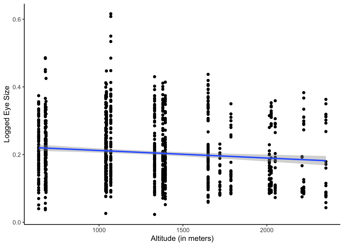
###/3 Test for Statistical Significance (Linear Regression)
mod_eye = lm(eye ~ altitude, data = Ant) #Creation of a linear model calculations for head measurements in relation to altitude
summary(mod_eye) #Displaying the results of the linear model calculation
Call:
lm(formula = eye ~ altitude, data = Ant)

Residuals:
     Min       1Q   Median       3Q      Max
-0.18512 -0.07062 -0.01803  0.06336  0.40555

Coefficients:
              Estimate Std. Error t value Pr(>|t|)
(Intercept)  2.343e-01  8.131e-03  28.814  < 2e-16 ***
altitude    -2.227e-05  5.992e-06  -3.716 0.000213 ***
---
Signif. codes:  0 '***' 0.001 '**' 0.01 '*' 0.05 '.' 0.1 ' ' 1

Residual standard error: 0.09223 on 1064 degrees of freedom
  (13 observations deleted due to missingness)
Multiple R-squared:  0.01281,   Adjusted R-squared:  0.01189
F-statistic: 13.81 on 1 and 1064 DF,  p-value: 0.0002126
:::
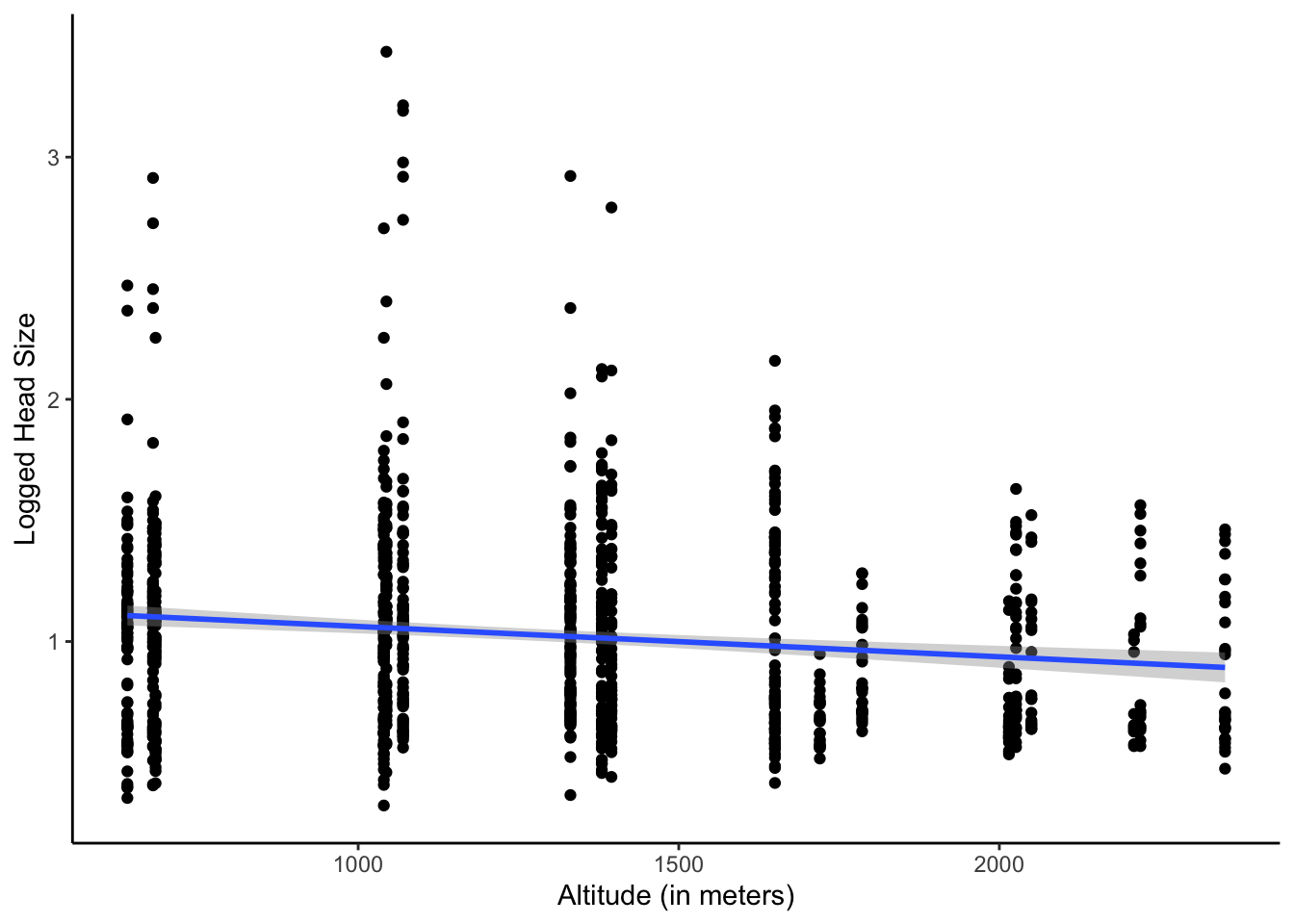
mod_head = lm(head ~ altitude, data = Ant) #Creation of a linear model calculations for head measurements in relation to altitude
summary(mod_head) #Displaying the results of the linear model calculation
Call:
lm(formula = head ~ altitude, data = Ant)

Residuals:
     Min       1Q   Median       3Q      Max
-0.75324 -0.29602 -0.04399  0.22126  2.37833

Coefficients:
              Estimate Std. Error t value Pr(>|t|)
(Intercept)  1.187e+00  3.613e-02  32.863  < 2e-16 ***
altitude    -1.252e-04  2.663e-05  -4.701 2.92e-06 ***
---
Signif. codes:  0 '***' 0.001 '**' 0.01 '*' 0.05 '.' 0.1 ' ' 1

Residual standard error: 0.4098 on 1064 degrees of freedom
  (13 observations deleted due to missingness)
Multiple R-squared:  0.02035,   Adjusted R-squared:  0.01943
F-statistic:  22.1 on 1 and 1064 DF,  p-value: 2.925e-06
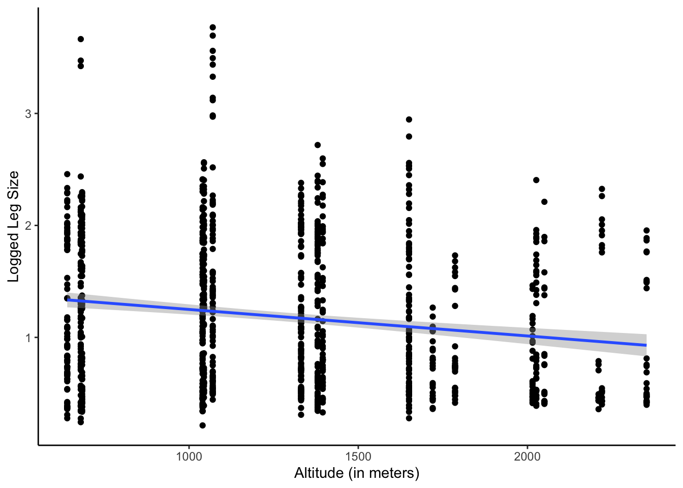
mod_leg = lm(leg ~ altitude, data = Ant) #Creation of a linear model calculations for head measurements in relation to altitude
summary(mod_leg) #Displaying the results of the linear model calculation
Call:
lm(formula = leg ~ altitude, data = Ant)

Residuals:
    Min      1Q  Median      3Q     Max
-1.0824 -0.5439 -0.1428  0.5350  2.5360

Coefficients:
              Estimate Std. Error t value Pr(>|t|)
(Intercept)  1.486e+00  5.796e-02  25.646  < 2e-16 ***
altitude    -2.368e-04  4.271e-05  -5.543 3.74e-08 ***
---
Signif. codes:  0 '***' 0.001 '**' 0.01 '*' 0.05 '.' 0.1 ' ' 1

Residual standard error: 0.6574 on 1064 degrees of freedom
  (13 observations deleted due to missingness)
Multiple R-squared:  0.02807,   Adjusted R-squared:  0.02716
F-statistic: 30.73 on 1 and 1064 DF,  p-value: 3.743e-08
mod_scape = lm(scape ~ altitude, data = Ant) #Creation of a linear model calculations for head measurements in relation to altitude
summary(mod_scape) #Displaying the results of the linear model calculation
Call:
lm(formula = scape ~ altitude, data = Ant)

Residuals:
     Min       1Q   Median       3Q      Max
-0.84836 -0.40154 -0.08094  0.40349  2.33945

Coefficients:
              Estimate Std. Error t value Pr(>|t|)
(Intercept)  1.324e+00  4.402e-02  30.087  < 2e-16 ***
altitude    -2.205e-04  3.244e-05  -6.796 1.78e-11 ***
---
Signif. codes:  0 '***' 0.001 '**' 0.01 '*' 0.05 '.' 0.1 ' ' 1

Residual standard error: 0.4993 on 1064 degrees of freedom
  (13 observations deleted due to missingness)
Multiple R-squared:  0.04161,   Adjusted R-squared:  0.04071
F-statistic: 46.19 on 1 and 1064 DF,  p-value: 1.783e-11
Result: All morphological features analyzed had a statistically significant relation to altitude (p-value < 0.05)
Figure Creation (Linear Regression)
# Linear regression figure for eye size
ggplot(Ant,aes(x=altitude, y=eye)) +
  geom_point() +
  theme_classic() + #Change theme  for aesthetics
  geom_smooth(method="lm") +
  labs(x='Altitude (in meters)', y='Logged Eye Size')
# Linear regression figure for head size
ggplot(Ant,aes(x=altitude, y=head)) +
  geom_point() +
  theme_classic() +
  geom_smooth(method="lm") +
  labs(x='Altitude (in meters)', y='Logged Head Size')
# Linear regression figure for leg size
ggplot(Ant,aes(x=altitude, y=leg)) +
  geom_point() +
  theme_classic() +
  geom_smooth(method="lm") +
  labs(x='Altitude (in meters)', y='Logged Leg Size')
# Linear regression figure for scape size
ggplot(Ant,aes(x=altitude, y=scape)) +
  geom_point() +
  theme_classic() +
  geom_smooth(method="lm") +
  labs(x='Altitude (in meters)', y='Logged Scape Size')
Result: Four figures depicting the relationship of ant morphology to altitude
TL;DR
This analysis is based on a several studies taking place in the Guadarra Mountains of Spain by the same group of scientists. Scientists measured the size of the different morphological structures of a multitude of ant genera across varying altitudes and regions of Guadarra mountain range as well as the resources ants were observed using. We aim to analyze how the size of the measured morphological features varies with altitude as well as to understand a genus-specific preference for certain resource types across ant taxa.